Tutorial 1: Disease diagnosis and biomarker identification

CellFreeGMF leverages machine learning and differential expression analysis to achieve diagnostic classification and biomarker identification for pancreatic ductal adenocarcinoma.

Preparation

import os
import numpy as np
import pandas as pd
from sklearn.model_selection import train_test_split
import shap
import matplotlib.pyplot as plt

import CellFreeGMF

Hyperparameter Configuration

current_path = os.path.abspath('')
disease_name = 'PDAC'

Load Data

def read_sample_cfRNA(disease_name = 'PDAC'):
    data_path = current_path + '/data/' + disease_name

    data_exp = pd.read_csv(data_path + '/GSE133684_exp_TPM-all.txt', sep='\t')
    data_exp = data_exp.set_index(data_exp.columns[0]).T

    label_all = pd.read_csv(data_path + '/GSE133684_series_matrix.csv', sep=',')

    label_all = label_all.set_index(label_all.columns[0])
    label_all['label'] = label_all[label_all.columns[0]].apply(lambda x: 1 if x == 'disease state: PDAC' else 0)

    # label_all = label_all.loc[data_exp.index]
    data_exp = data_exp.loc[label_all.index]

    data_all = {'data_exp': data_exp,
                'label': label_all}

    return data_all

# standardized matrix
def log_cpm(matrix: pd.DataFrame) -> pd.DataFrame:
    # Rows represent samples, and columns represent cfRNAs.
    matrix = matrix.T
    lib_size = matrix.sum(axis=0)
    cpm = matrix.divide(lib_size, axis=1) * 1e6
    log_cpm = np.log2(cpm + 1)
    return log_cpm.T

# read cfRNA data
sample_cfRNA_exp = read_sample_cfRNA(disease_name)
X_train, X_val, y_train, y_val = train_test_split(sample_cfRNA_exp['data_exp'], sample_cfRNA_exp['label']['label'], test_size=0.2, random_state=2025)

# Differential expression analysis was performed using the limma package.
DEG_res = CellFreeGMF.DEG_limma_fun(X_train, y_train, file_path = current_path + '/save_data/' + disease_name)

X_train = log_cpm(X_train)
X_val = log_cpm(X_val)

R[write to console]: 'select()' returned 1:many mapping between keys and columns

Diagnostic classification using machine learning was performed.

ML_lr, ML_lr_train, ML_lr_val, ML_lr_roc_ = CellFreeGMF.diagnosis_ML.ML_lr(X_train, y_train, X_val, y_val)
ML_svm, ML_svm_train, ML_svm_val, ML_svm_roc_  = CellFreeGMF.diagnosis_ML.ML_svm(X_train, y_train, X_val, y_val)
ML_rf, ML_rf_train, ML_rf_val, ML_rf_roc_ = CellFreeGMF.diagnosis_ML.ML_rf(X_train, y_train, X_val, y_val)
ML_ada, ML_ada_train, ML_ada_val, ML_ada_roc_ = CellFreeGMF.diagnosis_ML.ML_ada(X_train, y_train, X_val, y_val)
ML_dt, ML_dt_train, ML_dt_val, ML_dt_roc_ = CellFreeGMF.diagnosis_ML.ML_dt(X_train, y_train, X_val, y_val)
ML_knn, ML_knn_train, ML_knn_val, ML_knn_roc_ = CellFreeGMF.diagnosis_ML.ML_knn(X_train, y_train, X_val, y_val)

Logistic Regression:
Training dataset Accuracy: 1.0000, Precision: 1.0000, Recall: 1.0000, F1-Score: 1.0000, AUC:1.0000
Testing dataset Accuracy: 0.9383, Precision: 0.9387, Recall: 0.9383, F1-Score: 0.9368, AUC:0.9807
****************************************************************************************************
SVM:
Training dataset Accuracy: 0.7250, Precision: 0.8023, Recall: 0.7250, F1-Score: 0.6289, AUC:0.9954
Testing dataset Accuracy: 0.7284, Precision: 0.5306, Recall: 0.7284, F1-Score: 0.6139, AUC:0.9322
****************************************************************************************************
RandomForestClassifier:
Training dataset Accuracy: 1.0000, Precision: 1.0000, Recall: 1.0000, F1-Score: 1.0000, AUC:1.0000
Testing dataset Accuracy: 0.8642, Precision: 0.8720, Recall: 0.8642, F1-Score: 0.8515, AUC:0.9480
****************************************************************************************************
AdaBoostClassifier:
Training dataset Accuracy: 1.0000, Precision: 1.0000, Recall: 1.0000, F1-Score: 1.0000, AUC:1.0000
Testing dataset Accuracy: 0.9136, Precision: 0.9151, Recall: 0.9136, F1-Score: 0.9142, AUC:0.9769
****************************************************************************************************
DecisionTreeClassifier:
Training dataset Accuracy: 1.0000, Precision: 1.0000, Recall: 1.0000, F1-Score: 1.0000, AUC:1.0000
Testing dataset Accuracy: 0.7531, Precision: 0.7687, Recall: 0.7531, F1-Score: 0.7590, AUC:0.7165
****************************************************************************************************
KNeighborsClassifier:
Training dataset Accuracy: 0.7875, Precision: 0.7898, Recall: 0.7875, F1-Score: 0.7602, AUC:0.8920
Testing dataset Accuracy: 0.7407, Precision: 0.7073, Recall: 0.7407, F1-Score: 0.6992, AUC:0.6156
****************************************************************************************************

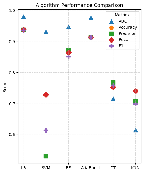
Performance comparison of diagnostic classification algorithms to screen for the algorithm optimally suited to PDAC.

# Algorithm names
algorithms = ['LR', 'SVM', 'RF', 'AdaBoost', 'DT', 'KNN']

# Evaluation metric scores for each algorithm.
metrics = {
    'AUC':      [ML_lr_val['auc_val'], ML_svm_val['auc_val'], ML_rf_val['auc_val'],ML_ada_val['auc_val'], ML_dt_val['auc_val'], ML_knn_val['auc_val']],
    'Accuracy': [ML_lr_val['accuracy_val'], ML_svm_val['accuracy_val'], ML_rf_val['accuracy_val'],ML_ada_val['accuracy_val'], ML_dt_val['accuracy_val'], ML_knn_val['accuracy_val']],
    'Precision':[ML_lr_val['precision_val'], ML_svm_val['precision_val'], ML_rf_val['precision_val'],ML_ada_val['precision_val'], ML_dt_val['precision_val'], ML_knn_val['precision_val']],
    'Recall':   [ML_lr_val['recall_val'], ML_svm_val['recall_val'], ML_rf_val['recall_val'],ML_ada_val['recall_val'], ML_dt_val['recall_val'], ML_knn_val['recall_val']],
    'F1':       [ML_lr_val['f1_val'], ML_svm_val['f1_val'], ML_rf_val['f1_val'],ML_ada_val['f1_val'], ML_dt_val['f1_val'], ML_knn_val['f1_val']]
}

# Assign a distinct marker shape to each evaluation metric.
markers = {
    'AUC': '^',          # triangle
    'Accuracy': 'o',     # circle
    'Precision': 's',    # square
    'Recall': 'D',       # diamond
    'F1': 'P'            # pentagon
}

# plot
plt.figure(figsize=(5, 6))

# The x-axis denotes the algorithms.
x = np.arange(len(algorithms))

# Plot scatter points
for metric, scores in metrics.items():
    plt.scatter(x, scores, label=metric, marker=markers[metric], s=100)

# Set the legend, labels, and axes.
plt.xticks(x, algorithms)
plt.ylabel("Score")
plt.title("Algorithm Performance Comparison")
plt.legend(title="Metrics")
plt.grid(True, linestyle='--', alpha=0.5)

plt.tight_layout()

# Save as PDF
plt.savefig(current_path + '/save_data/' + disease_name + "/Fig2a.pdf")

plt.show()
plt.close()

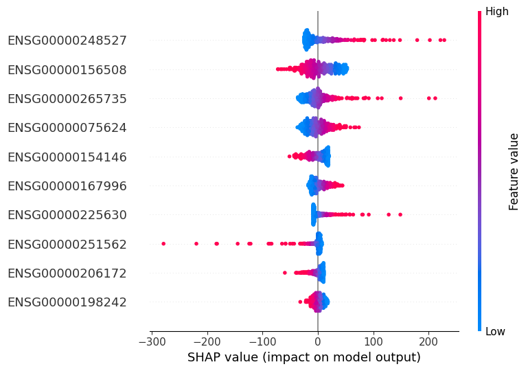
The optimal logistic regression model was selected and subsequently retrained on the full dataset; interpretability analysis was then performed to identify candidate target cfRNAs.

X = sample_cfRNA_exp['data_exp']
ML_lr = CellFreeGMF.diagnosis_ML.ML_lr(sample_cfRNA_exp['data_exp'], sample_cfRNA_exp['label']['label'])

Logistic Regression:
Training dataset Accuracy: 1.0000, Precision: 1.0000, Recall: 1.0000, F1-Score: 1.0000, AUC:1.0000
****************************************************************************************************

SHAP-based interpretability analysis

explainer = shap.LinearExplainer(ML_lr, X, feature_names=X.columns)
shap_values = explainer(X)

shap.summary_plot(shap_values, X, feature_names=X.columns, show=False, max_display=10)

Save the differential expression analysis results and the SHAP results.

save SHAP result

# extract feature importance
shap_importance = np.abs(shap_values.values).mean(axis=0)
feature_names = X.columns

importance_df = pd.DataFrame({
    'Feature': X.columns,
    'Mean_ABS_SHAP': shap_importance
})

importance_df = importance_df.sort_values(by='Mean_ABS_SHAP', ascending=False)
importance_df.to_csv(current_path + '/save_data/' + disease_name + '/shap_feature_importance.csv', index=False)

# the top 10% in terms of importance were selected
sorted_idx = np.argsort(shap_importance)[::-1]

feature_names[sorted_idx[:round(sorted_idx.size * 0.1)]].to_series().to_csv(current_path + '/save_data/' + disease_name + '/SHAP_ALL_gene.txt', header=False, index=False)
pd.DataFrame({
    'gene_id': feature_names[sorted_idx],
    'feature_importance': shap_importance[sorted_idx]
}).to_csv(current_path + '/save_data/' + disease_name + '/SHAP_results.csv', header=False, index=False)

save DEG result

DEG_res.to_csv(current_path + '/save_data/' + disease_name + '/DEG_res.csv')